Nodal Analysis

Objective:

The objective for this lab was to determine voltages across resistors, in a circuit with two voltage sources, using nodal analysis. Nodal analysis is necessary to find the power that the resistors should be able to handle if both batteries are on. This is what the circuit looked like.

Procedure:

1. First we assigned node voltages and found the governing nodal equations for the circuit.

2. We then solved for the unknown node voltages across the resistors.

Introduction to Biasing

Objective:
The purpose of this lab was to find appropriate biasing resistors so that two LEDs would light up within their power ratings. Applying KCL and KVL to the circuit and adjusting the calculated resistances to practical resistor values will make the circuit operate correctly.

Procedure:

First we modeled the circuit to be used and calculated what the maximum resistances across the LEDs should be.
R_led1= 5V/0.02275A = 219.78 ohms
R_led2= 2V/0.02A = 100 ohms









Then we could find the minimum resistances R1 and R2 from the maximum current and LED voltages from the circuit.

As a practical matter we chose to use:

R1=150 ohms + 40 ohms =190 ohms
R2=360 ohms

Here was the circuit incarnate:









The data revealed some interesting behaviors. Removing one LED would raise the voltage and current of the other resistor.

Conclusion:
We were able to bias the circuit successfully to light both LEDs with a 9V source. According to my efficiency equation the minimum voltage to power the LEDs  in the Figure 2 configuration would be 3.6V. The answers to the final questions are below.

FreeMat: Introduction to Numerical Computation

Solving Simultaneous Equations:

Assignment 1

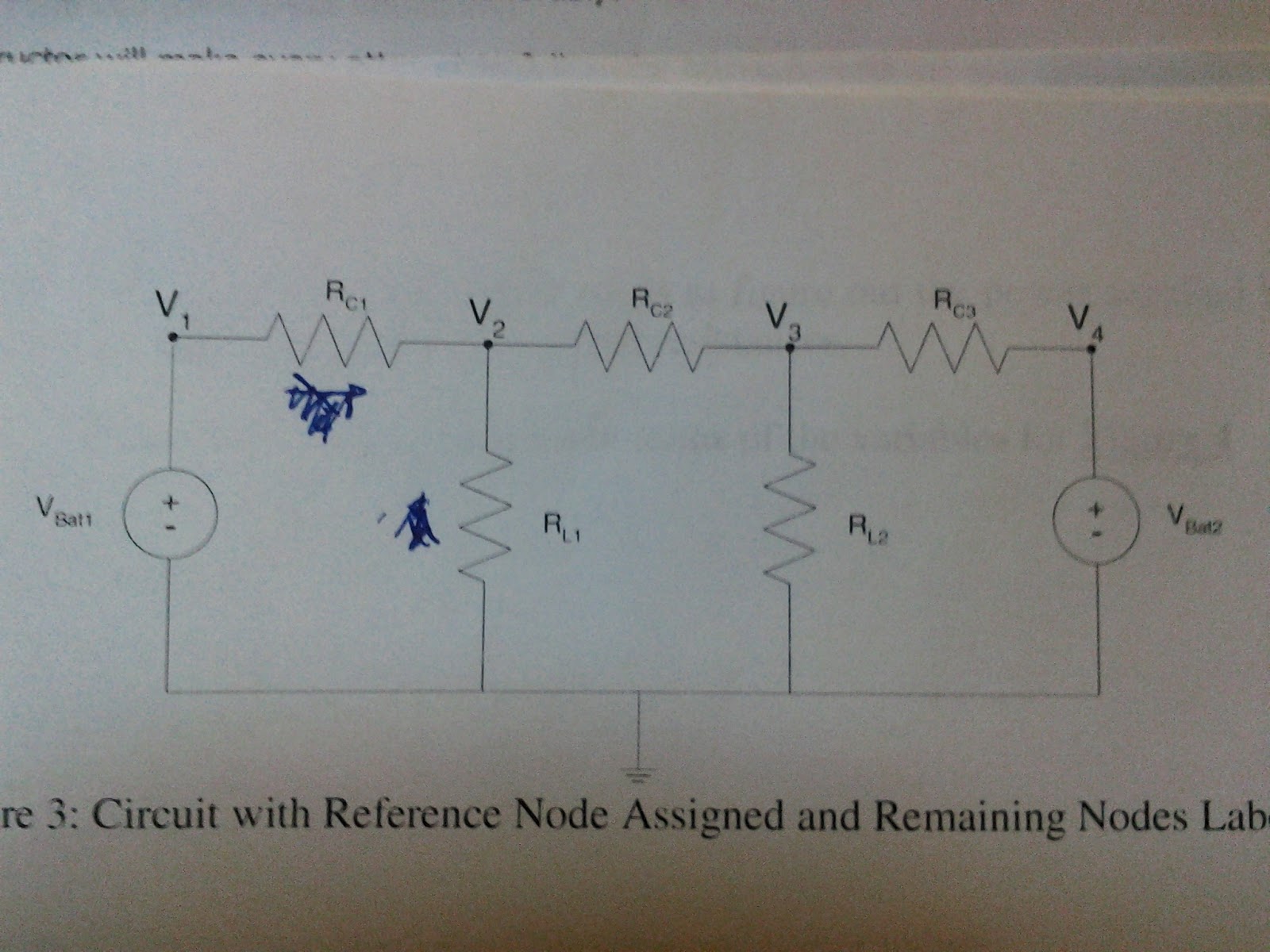
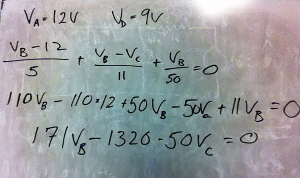
To solve the system of equations derived from this circuit I used KCL and KVL. 

See the derivation and diagram below.

I created simple matrices with respect to current, voltage, and resistance in FreeMat to solve for the current across R_3.

Adding Sinusoids:

Assignment 1

1. Circuit A has a time constant of 100 ms, while circuit B  has a time constant of 200 ms. The circuit output is 2e^(-t/tau).

Circuit outputs generated by FreeMat were graphed for circuits A and B as the blue and green curves respectively.

From this graph it shows that circuit A reaches a lower output sooner.

2. If the circuit's output is related to 2(1-e(-t/tau)) the FreeMat generates the graph below.

In this case, circuit A-in blue-would also reach its maximum output sooner than circuit B.

Assignment 2

1. The output generated by the sum of two sinusoidal functions was found theoretically and through FreeMat. FreeMat also graphed the result of both methods to compare directly.

f1: blue

f2: green

F: red

This is the result of the theoretical function which matches exactly to that of the first method.

2. For a frequency of 10 Hz the process of plotting the graph was very similar except that the period is much shorter.

Introduction to DC Circuits Lab

Objective
The purpose of this lab was to find the most efficient circuit to deliver power to a load with an unknown length of AWG #30 cable. To find the optimal length of cable and load system we set up the lab equipment in a circuit as shown:

This is how the circuit looked when assembled.

Theoretically the load of the circuit would need to be 1000 ohms and receive a voltage of at least 11V.

However the actual resistance of the load was smaller.

According to the DMMs and calculations for length the maximum resistance the cable could sustain while maintaining 11V across the load was 83 ohms with a distance of 120.25m of AWG #30 cable.

The distribution efficiency was calculated as a function of the power out and power lost during the experiment. The values of the powers were calculated using the measurments from the DMMs in our setup. The distribution efficiency came out to be 92.1% and the calculated average time to discharge by the battery was 4.24 minutes.

Times to Discharge:

9.71s

9.69s

9.74s

9.72s

Conclusion:

A submarine with a power absorption of 0.1238W would be able to travel with up to 120.25m of AWG #30 cable provided that it would also be able to carry the weight of the cable in the water. With a 92.1% distribution efficiency, the submarine would also be able to operate for more than 4 minutes-- enough time to perform accurate maneuvers.